Preparation for Group Assignment

Preparation for Group Assignment#

This tutorial contains various small guides for tasks you will need or come in handy in the upcoming group assignment.

We’re going to need a couple of packages for this tutorial:

from atlite.gis import ExclusionContainer
from atlite.gis import shape_availability
import atlite
import rasterio as rio
from rasterio.plot import show
import geopandas as gpd
import pandas as pd
import numpy as np
import xarray as xr
import os
import matplotlib.pyplot as plt
import country_converter as coco
import atlite

Preparatory Downloads#

For this tutorial, we also need to download a few files, for which one can use the urllib library:

Downloading historical weather data from ERA5 with `atlite`#

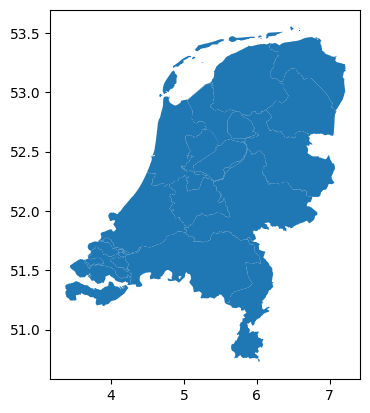
First, let’s load some small example country. Let’s say, the Netherlands.

fn = "https://tubcloud.tu-berlin.de/s/567ckizz2Y6RLQq/download?path=%2Fgadm&files=gadm_410-levels-ADM_1-NLD.gpkg"
regions = gpd.read_file(fn)

/opt/hostedtoolcache/Python/3.11.9/x64/lib/python3.11/site-packages/pyogrio/raw.py:196: RuntimeWarning: File /vsimem/82ae5577b3fd409f8a3171f9abab23cc has GPKG application_id, but non conformant file extension
  return ogr_read(

regions.plot()

<Axes: >

../_images/9c002fdd67367a9a6682c9bdae5082a350b3c7e74216063a819d44edda6c2b06.png

In this example we download historical weather data ERA5 data on-demand for a cutout we want to create.

Note

For this example to work, you should have

installed the Copernicus Climate Data Store cdsapi package (conda list cdsapi or pip install cdsapi) and
registered and setup your CDS API key as described on this website. Note that there are different instructions depending on your operating system.

A cutout is the basis for any of your work and calculations in atlite.

The cutout is created in the directory and file specified by the relative path. If a cutout at the given location already exists, then this command will simply load the cutout again. If the cutout does not yet exist, it will specify the new cutout to be created.

For creating the cutout, you need to specify the dataset (e.g. ERA5), a time period and the spatial extent (in latitude and longitude).

minx, miny, maxx, maxy = regions.total_bounds
buffer = 0.25

cutout = atlite.Cutout(
    path="era5-2013-NL.nc",
    module="era5",
    x=slice(minx - buffer, maxx + buffer),
    y=slice(miny - buffer, maxy + buffer),
    time="2013",
)

/opt/hostedtoolcache/Python/3.11.9/x64/lib/python3.11/site-packages/atlite/cutout.py:191: UserWarning: Arguments module, x, y, time are ignored, since cutout is already built.
  warn(

Calling the function cutout.prepare() initiates the download and processing of the weather data. Because the download needs to be provided by the CDS servers, this might take a while depending on the amount of data requested.

Note

You can check the status of your request here.

cutout.prepare()

---------------------------------------------------------------------------
Exception                                 Traceback (most recent call last)
Cell In[11], line 1
----> 1 cutout.prepare()

File /opt/hostedtoolcache/Python/3.11.9/x64/lib/python3.11/site-packages/atlite/data.py:103, in maybe_remove_tmpdir.<locals>.wrapper(*args, **kwargs)
    101 kwargs["tmpdir"] = mkdtemp()
    102 try:
--> 103     res = func(*args, **kwargs)
    104 finally:
    105     rmtree(kwargs["tmpdir"])

File /opt/hostedtoolcache/Python/3.11.9/x64/lib/python3.11/site-packages/atlite/data.py:177, in cutout_prepare(cutout, features, tmpdir, overwrite, compression)
    175 logger.info(f"Calculating and writing with module {module}:")
    176 missing_features = missing_vars.index.unique("feature")
--> 177 ds = get_features(cutout, module, missing_features, tmpdir=tmpdir)
    178 prepared |= set(missing_features)
    180 cutout.data.attrs.update(dict(prepared_features=list(prepared)))

File /opt/hostedtoolcache/Python/3.11.9/x64/lib/python3.11/site-packages/atlite/data.py:46, in get_features(cutout, module, features, tmpdir)
     41     feature_data = delayed(get_data)(
     42         cutout, feature, tmpdir=tmpdir, lock=lock, **parameters
     43     )
     44     datasets.append(feature_data)
---> 46 datasets = compute(*datasets)
     48 ds = xr.merge(datasets, compat="equals")
     49 for v in ds:

File /opt/hostedtoolcache/Python/3.11.9/x64/lib/python3.11/site-packages/dask/base.py:662, in compute(traverse, optimize_graph, scheduler, get, *args, **kwargs)
    659     postcomputes.append(x.__dask_postcompute__())
    661 with shorten_traceback():
--> 662     results = schedule(dsk, keys, **kwargs)
    664 return repack([f(r, *a) for r, (f, a) in zip(results, postcomputes)])

File /opt/hostedtoolcache/Python/3.11.9/x64/lib/python3.11/site-packages/atlite/datasets/era5.py:417, in get_data(cutout, feature, tmpdir, lock, **creation_parameters)
    413     return retrieve_once(retrieval_times(coords, static=True)).squeeze()
    415 datasets = map(retrieve_once, retrieval_times(coords))
--> 417 return xr.concat(datasets, dim="time").sel(time=coords["time"])

File /opt/hostedtoolcache/Python/3.11.9/x64/lib/python3.11/site-packages/xarray/core/concat.py:254, in concat(objs, dim, data_vars, coords, compat, positions, fill_value, join, combine_attrs, create_index_for_new_dim)
    251 from xarray.core.dataset import Dataset
    253 try:
--> 254     first_obj, objs = utils.peek_at(objs)
    255 except StopIteration:
    256     raise ValueError("must supply at least one object to concatenate")

File /opt/hostedtoolcache/Python/3.11.9/x64/lib/python3.11/site-packages/xarray/core/utils.py:198, in peek_at(iterable)
    194 """Returns the first value from iterable, as well as a new iterator with
    195 the same content as the original iterable
    196 """
    197 gen = iter(iterable)
--> 198 peek = next(gen)
    199 return peek, itertools.chain([peek], gen)

File /opt/hostedtoolcache/Python/3.11.9/x64/lib/python3.11/site-packages/atlite/datasets/era5.py:407, in get_data.<locals>.retrieve_once(time)
    406 def retrieve_once(time):
--> 407     ds = func({**retrieval_params, **time})
    408     if sanitize and sanitize_func is not None:
    409         ds = sanitize_func(ds)

File /opt/hostedtoolcache/Python/3.11.9/x64/lib/python3.11/site-packages/atlite/datasets/era5.py:201, in get_data_temperature(retrieval_params)
    197 def get_data_temperature(retrieval_params):
    198     """
    199     Get wind temperature for given retrieval parameters.
    200     """
--> 201     ds = retrieve_data(
    202         variable=[
    203             "2m_temperature",
    204             "soil_temperature_level_4",
    205             "2m_dewpoint_temperature",
    206         ],
    207         **retrieval_params,
    208     )
    210     ds = _rename_and_clean_coords(ds)
    211     ds = ds.rename(
    212         {
    213             "t2m": "temperature",
   (...)
    216         }
    217     )

File /opt/hostedtoolcache/Python/3.11.9/x64/lib/python3.11/site-packages/atlite/datasets/era5.py:328, in retrieve_data(product, chunks, tmpdir, lock, **updates)
    322 request.update(updates)
    324 assert {"year", "month", "variable"}.issubset(
    325     request
    326 ), "Need to specify at least 'variable', 'year' and 'month'"
--> 328 client = cdsapi.Client(
    329     info_callback=logger.debug, debug=logging.DEBUG >= logging.root.level
    330 )
    331 result = client.retrieve(product, request)
    333 if lock is None:

File /opt/hostedtoolcache/Python/3.11.9/x64/lib/python3.11/site-packages/cdsapi/api.py:281, in Client.__new__(cls, url, key, *args, **kwargs)
    280 def __new__(cls, url=None, key=None, *args, **kwargs):
--> 281     _, token, _ = get_url_key_verify(url, key, None)
    282     if ":" in token:
    283         return super().__new__(cls)

File /opt/hostedtoolcache/Python/3.11.9/x64/lib/python3.11/site-packages/cdsapi/api.py:69, in get_url_key_verify(url, key, verify)
     66             verify = bool(int(config.get("verify", 1)))
     68 if url is None or key is None or key is None:
---> 69     raise Exception("Missing/incomplete configuration file: %s" % (dotrc))
     71 # If verify is still None, then we set to default value of True
     72 if verify is None:

Exception: Missing/incomplete configuration file: /home/runner/.cdsapirc

The data is accessible in cutout.data. Included weather variables are listed in cutout.prepared_features. Querying the cutout gives us some basic information on which data is contained in it.

cutout.data

cutout.prepared_features

cutout

Repetition: From Land Eligibility Analysis to Availability Matrix#

We’re going to use the plotting functions from previous exercises:

def plot_area(masked, transform, shape):
    fig, ax = plt.subplots(figsize=(5, 5))
    ax = show(masked, transform=transform, cmap="Greens", vmin=0, ax=ax)
    shape.plot(ax=ax, edgecolor="k", color="None", linewidth=1)

First, we collect all exclusion and inclusion criteria in an ExclusionContainer.

excluder = ExclusionContainer(crs=3035, res=300)
fn = "PROBAV_LC100_global_v3.0.1_2019-nrt_Discrete-Classification-map_EPSG-4326-NL.tif"
excluder.add_raster(fn, codes=[50], buffer=1000, crs=4326)
excluder.add_raster(fn, codes=[20, 30, 40, 60], crs=4326, invert=True)
fn = "WDPA_Oct2022_Public_shp-NLD.tif"
excluder.add_raster(fn, crs=3035)
fn = "GEBCO_2014_2D-NL.nc"
excluder.add_raster(fn, codes=lambda x: x > 10, crs=4326, invert=True)

Then, we can calculate the available areas…

masked, transform = shape_availability(regions.to_crs(3035).geometry, excluder)

… and plot it:

plot_area(masked, transform, regions.to_crs(3035).geometry)

Availability Matrix#

regions.index = regions.GID_1

cutout = atlite.Cutout("era5-2013-NL.nc")

?cutout.availabilitymatrix

A = cutout.availabilitymatrix(regions, excluder)

cap_per_sqkm = 1.7  # MW/km2

area = cutout.grid.set_index(["y", "x"]).to_crs(3035).area / 1e6

area = xr.DataArray(area, dims=("spatial"))

capacity_matrix = A.stack(spatial=["y", "x"]) * area * cap_per_sqkm

Solar PV Profiles#

pv = cutout.pv(
    panel=atlite.solarpanels.CdTe,
    matrix=capacity_matrix,
    orientation="latitude_optimal",
    index=regions.index,
    per_unit=True,
)

pv.to_pandas().head()

pv.to_pandas().iloc[:, 0].plot()

Wind Profiles#

wind = cutout.wind(
    atlite.windturbines.Vestas_V112_3MW,
    matrix=capacity_matrix,
    index=regions.index,
    per_unit=True,
)

wind.to_pandas().head()

wind.to_pandas().iloc[:, 0].plot()

Merging Shapes in `geopandas`#

Spatial data is often more granular than we need. For example, we might have data on sub-national units, but we’re actually interested in studying patterns at the level of countries.

Whereas in pandas we would use the groupby() function to aggregate entries, in geopandas, we aggregate geometric features using the dissolve() function.

Suppose we are interested in studying continents, but we only have country-level data like the country dataset included in geopandas. We can easily convert this to a continent-level dataset.

Note

world = gpd.read_file(gpd.datasets.get_path("naturalearth_lowres"))

world.head(3)

continents = world.dissolve(by="continent").geometry

continents.plot();

If we are interested in the population per continent, we can pass different aggregation strategies to the dissolve() functionusing the aggfunc argument:

https://geopandas.org/en/stable/docs/user_guide/aggregation_with_dissolve.html#dissolve-arguments

continents = world.dissolve(by="continent", aggfunc=dict(pop_est="sum"))

continents.plot(column="pop_est");

You can also pass a pandas.Series to the dissolve() function that describes your mapping for more exotic aggregation strategies (e.g. by first letter of the country name):

world.dissolve(by=world.name.str[0], aggfunc=dict(pop_est="sum")).plot(column="pop_est")

Representative Points and Crow-Fly Distances#

The following example includes code to retrieve representative points from polygons and to calculate the distance on a sphere between two points.

Note

world = gpd.read_file(gpd.datasets.get_path("naturalearth_lowres"))

points = world.representative_point()

fig, ax = plt.subplots()
world.plot(ax=ax)
points.plot(ax=ax, color="red", markersize=3);

points = points.to_crs(4087)
points.index = world.iso_a3

distances = pd.concat({k: points.distance(p) for k, p in points.items()}, axis=1).div(
    1e3
)  # km

distances.loc["DEU", "NLD"]

cutout.data.temperature.sel(time="2013-01-01 00:00").to_pandas().head()

Global Equal-Area and Equal-Distance CRS#

Previously, we used EPSG:3035 as projection to calculate the area of regions in km². However, this projection is not correct for regions outside of Europe, so that we need to pick different, more suitable projections for calculating areas and distances between regions.

for calculating distances: WGS 84 / World Equidistant Cylindrical (EPSG:4087)
for calculating areas: Mollweide (ESRI:54009)

The unit of measurement for both projections is metres.

AREA_CRS = "ESRI:54009"
DISTANCE_CRS = "EPSG:4087"

world = gpd.read_file(gpd.datasets.get_path("naturalearth_lowres"))

world.to_crs(AREA_CRS).plot()

world.to_crs(DISTANCE_CRS).plot()

Country Converter#

The country converter (coco) is a Python package to convert and match country names between different classifications and between different naming versions.

Note

import country_converter as coco

Convert various country names to some standard names, specifying source and target classification scheme:

coco.convert(names="NLD", to="name_official")

coco.convert(names="NLD", to="iso2")

coco.convert(names="NLD", src="iso3", to="iso2")

country_list = ["AE", "AL", "AM", "AO", "AR"]

coco.convert(names=country_list, src="iso2", to="short_name")

List of included country classification schemes:

cc = coco.CountryConverter()
cc.valid_country_classifications

Gurobi#

Gurobi is one of the most powerful solvers to solve optimisation problems. It is a commercial solver, with free academic licenses.

Note

Using this solver for the group assignment is optional. You can also use other open-source alternatives, but they might just take a little longer to solve.

To set up Gurobi, you need to:

Register at https://pages.gurobi.com/registration/ with your institutional e-mail address (e.g. @campus.tu-berlin.de).
Follow the getting started guide for your respective operating system at https://www.gurobi.com/documentation/quickstart.html (this includes a guide for retrieving your academic license and installing the software).
In your conda environment, install gurobipy with pip install gurobipy.

Preparation for Group Assignment

Contents

Preparation for Group Assignment#

Preparatory Downloads#

Downloading historical weather data from ERA5 with atlite#

Repetition: From Land Eligibility Analysis to Availability Matrix#

Availability Matrix#

Solar PV Profiles#

Wind Profiles#

Merging Shapes in geopandas#

Representative Points and Crow-Fly Distances#

Global Equal-Area and Equal-Distance CRS#

Country Converter#

Gurobi#

Downloading historical weather data from ERA5 with `atlite`#

Merging Shapes in `geopandas`#